How to analyze Force-Volume images?
How to analyze Force-Volume images?
PUNIAS can also be used to analyze so called FV (Force-Volume) files, which are images composed of arrays of single force curves.
In the case you are using and starting PUNIAS for the first time, please read first the section How to use PUNIAS.
To start the analysis, a batch file can be generated and opened, the force curves opened directly, or the force curves opened through a drag & drop process.
PUNIAS will then open (one after the other) all the curves to be analyzed. After plotting the curve, as force versus extension or deformation, the computer determines the best possible baseline for the corresponding curve, and adds it to the graph. In the same way, the unfolding peaks or markers for the different calculations are determined by an algorithm and plotted on the graph. With all of these results being plotted on the graph along with the experimental curve, the user can very quickly visualize the results the computer finds, and validate them by saving the results and moving to the next file.

In case the user erroneously proceeds to the next file, he or she may go back (maximum 5 files) and re-analyze them by using the Home key. In case the user disagrees with the results of the algorithm, it is possible for the user to place a different baseline. The choice of a new baseline will discard all the unfolding peaks or markers found previously and generate a new set of results corresponding to the parameters characterized by the value of the new baseline. Once the user agrees with the setting of the baseline, it is then possible to add or discard peaks or modify the position of the markers. All the manual interactions with the software are done through the mouse and the keyboard using the arrow-keys and programmed keys.
A convenient way to obtain information on any part of the software is to use the contextual help: 
The data is serialized immediately after each file is analyzed to avoid data loss.
A result file data file (extension .pic) is generated with the name of the file followed by different information depending on the type of analysis used.
All the data obtained at the end of the analysis can then be opened by different ASCII software to plot histograms and perform further analysis
Also, ASCII files can be created (if the Save ASCII Files option is activated) for each file opened to simplify the plotting of the files with spreadsheet software. These files are saved in a folder named PlotableData and contain four columns (piezo position for extension, extension curve, piezo position for retraction, retraction curve) with the data expressed in nanometers. And in the case of nano-indentation, there are additional ASCII files saved in a folder nanoIndent and containing four columns (deformation for extension and retraction in nanometer and force in pico Newton).
A FV image is composed of several thousand of single force curves and it is thus impossible to manually go through and analyze them. Because of this, we have implemented an automatic analysis feature that will automatically open and analyze all the force curves indicated in the batch file.

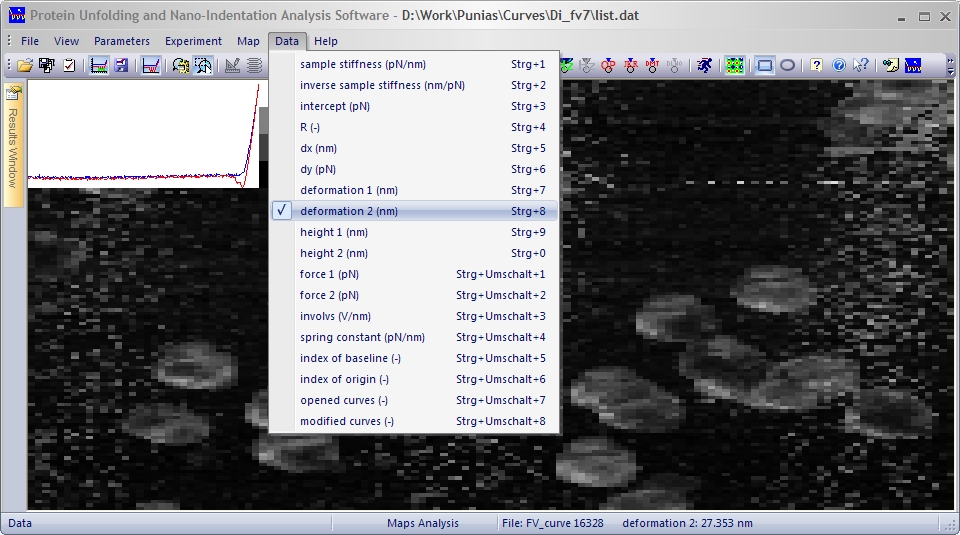
Once all the files have been analyzed, the map of the analyzed results can be visualized. In order to do this, the Maps Analysis (3D) has to be activated.

Then Open the previously generated batch file in order to visualize the maps.


Each time a different map is selected, a data file (extension .map) is saved in the data folder with all the data of the map in a format that can be easily imported in spreadsheet software.
All the data of the result file that can thus be visualized as a map and exported:
Additionally to the map a results window displaying all the results data of a given curve can be visualized or not:

The main with the analysis method described so far is that when letting an automatic algorithm perform an analysis, only at the most 70 to 80 % of the curves are correctly analyzed. Thus it may be necessary to "manually" check how the algorithm has evaluated some of the most critical curves.
When double clicking on a position on the map, the corresponding curve will be displayed with the previously saved analysis settings. The user has then the possibility to modify the settings.

When doing so, a new map file (extension .map) will be saved with the updated data, as well as a new result file (extension .mip), which is similar to the opened result file with the updated data.
Sometimes it may be necessary to select several curves on the map to be reanalyzed. This can be done by right clicking on the map and dragging a ROI (Region Of Interest):

Once a ROI has been selected, the reanalysis of all the selected curves can be launched:

Similar to the single curves reanalysis described before, a new map file (extension .map) will be saved with the updated data, as well as a new result file (extension .mip), which is similar to the opened result file with the updated data.
Additionally and when the Save ROI option has been activated a new result file (extension .roi), of all the curves in the ROI will be saved with the updated data in a format similar to the to the opened result file (extension .pic).

The analysis of the selected curves in the ROI can be cancelled by clicking again on the launch analysis button.
For any questions, suggestions, corrections, and requests for information please send a mail to: punias@free.fr.